
The natural world is a tapestry woven with countless threads of life, each species a unique color or texture. When we speak of biodiversity, we often first think of the sheer number of species found in a single place, like the dazzling array of insects in a rainforest or the diverse fish in a coral reef. This local richness is a crucial aspect of biodiversity, but it tells only part of the story. To truly appreciate the complexity and interconnectedness of life on Earth, we must also consider how species composition changes from one place to another. This spatial dimension of biodiversity is precisely what “beta diversity” helps us understand.
Unpacking Biodiversity: Alpha and Beta Diversity
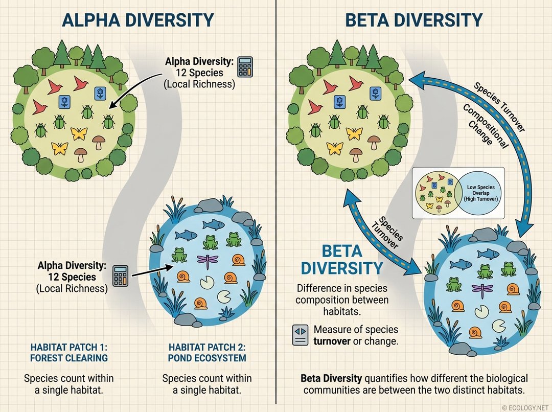
Before diving deep into beta diversity, it is helpful to distinguish it from its close relative, alpha diversity.
- Alpha Diversity: This refers to the species richness within a single, defined habitat or community. Imagine counting all the different types of birds you see in your backyard over a month, or all the plant species in a specific meadow. That count represents the alpha diversity of that particular location. It is a measure of local diversity.
- Beta Diversity: This is where the spatial element comes into play. Beta diversity measures the difference in species composition between two or more different habitats or communities. It quantifies the “species turnover” as you move from one place to another. If your backyard has robins and sparrows, but a nearby forest has owls and woodpeckers, the difference in those bird communities is a reflection of beta diversity.
Think of it this way: alpha diversity is about how many unique species are in one room, while beta diversity is about how different the species in one room are compared to the species in another room.
Why Beta Diversity is Indispensable
Understanding beta diversity is not merely an academic exercise; it is fundamental for effective conservation, ecological research, and environmental management. Here is why it holds such significant importance:
- Revealing Ecological Patterns: Beta diversity helps ecologists understand the processes that shape communities. It can indicate how species respond to environmental changes, how dispersal limitations affect distribution, and how different species interact across landscapes.
- Informing Conservation Strategies: When prioritizing areas for protection, knowing only alpha diversity can be misleading. A region might have many sites with high alpha diversity, but if all those sites share largely the same species, protecting just one might be sufficient for those species. However, if there is high beta diversity, meaning each site has a unique set of species, then protecting multiple sites becomes crucial to conserve the full spectrum of regional biodiversity. It helps identify unique habitats and hotspots of species turnover.
- Assessing Environmental Impact: Changes in beta diversity can signal environmental degradation or recovery. For instance, habitat fragmentation can increase beta diversity by isolating populations and preventing species movement, or it can decrease it if generalist species dominate across fragmented patches, leading to homogenization.
- Guiding Restoration Efforts: For ecological restoration projects, understanding the historical or target beta diversity can help guide species reintroductions and habitat reconstruction to ensure the restored area contributes meaningfully to regional biodiversity.
The Architects of Species Turnover: Drivers of Beta Diversity
What causes species composition to vary from one place to another? A multitude of factors, both environmental and historical, sculpt the patterns of beta diversity we observe in nature.
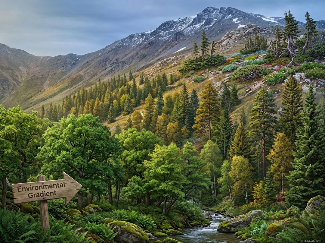
Environmental Gradients: Nature’s Shifting Canvas
One of the most powerful drivers of beta diversity is the presence of environmental gradients. These are gradual changes in environmental conditions across a landscape, such as temperature, moisture, elevation, soil type, or salinity. As these conditions change, so do the species best adapted to thrive in those specific circumstances.
Consider a mountain slope, a classic example of an environmental gradient:
- At the base, where temperatures are warmer and moisture is abundant, you might find lush broadleaf forests with a particular set of understory plants and animals.
- As you ascend, temperatures drop, and conditions become harsher. The broadleaf trees might give way to mixed forests, then to coniferous trees, each supporting a different array of species.
- Near the summit, you might encounter hardy alpine shrubs, grasses, and specialized rock-dwelling organisms, a completely distinct community from the base.
The continuous change in species composition as you move up the mountain is a direct manifestation of beta diversity driven by the elevational gradient.
Other examples of environmental gradients include:
- Riparian zones: The transition from a river channel to the dry land, with distinct communities adapted to varying water levels.
- Intertidal zones: The area between high and low tide marks, where organisms face extreme fluctuations in submersion and exposure.
- Soil nutrient gradients: Different plant communities thrive on nutrient-rich versus nutrient-poor soils.
Habitat Heterogeneity: The Mosaic of Life
Even within a seemingly uniform area, variations in microhabitats can create significant beta diversity. A forest, for example, might contain patches of dense canopy, sun-dappled clearings, fallen logs, and small streams. Each of these microhabitats can support a unique subset of species, contributing to the overall beta diversity of the larger forest ecosystem.
Geographic Distance and Dispersal Limitation: The Barriers to Movement
Simply put, species cannot be everywhere. The further apart two habitats are, the less likely they are to share species, especially if there are barriers to dispersal like mountains, oceans, or human-modified landscapes. This “distance decay” in similarity is a common pattern in beta diversity studies. The classic theory of island biogeography, for instance, highlights how isolation limits the colonization of new species, leading to distinct communities on different islands.
Historical and Evolutionary Factors: Echoes of the Past
The geological and evolutionary history of a region also plays a profound role. Past glaciations, continental drift, volcanic activity, or long periods of isolation can lead to the evolution of unique species in different areas, contributing to high beta diversity even in similar present-day environments.
Species Interactions: The Web of Life
Competition, predation, mutualism, and other interactions between species can also influence local community composition and, consequently, beta diversity. For example, the presence of a dominant competitor in one habitat might exclude certain species that are present in a neighboring habitat where the competitor is absent.
Quantifying the Difference: Measuring Beta Diversity
To move beyond qualitative descriptions, ecologists employ various indices to quantify beta diversity. These mathematical tools allow for rigorous comparison of communities and the detection of patterns across landscapes. One of the most widely used and intuitive measures is the Jaccard Index.
The Jaccard Index: A Simple Comparison
The Jaccard Index (J) measures the similarity between two communities based on the presence or absence of species. It is calculated as the number of species shared between the two communities, divided by the total number of unique species found across both communities.
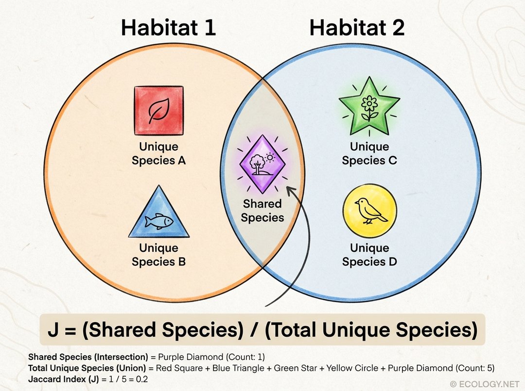
The formula is typically expressed as:
J = C / (A + B + C)
- A: The number of species unique to Habitat 1.
- B: The number of species unique to Habitat 2.
- C: The number of species shared by both Habitat 1 and Habitat 2.
A Jaccard Index value ranges from 0 to 1:
- A value of 1 indicates perfect similarity (the two habitats share all their species).
- A value of 0 indicates no similarity (the two habitats share no species).
To express beta diversity as a dissimilarity, you can simply calculate 1 – Jaccard Index. A higher dissimilarity value means greater beta diversity.
While the Jaccard Index is popular, other indices exist, such as the Sørensen Index (which gives more weight to shared species) and various measures that account for species abundance rather than just presence/absence. The choice of index often depends on the specific research question and the nature of the data.
Beyond Simple Turnover: Nestedness and Replacement
Modern approaches to beta diversity often decompose it into two main components: species replacement (or turnover) and nestedness. This distinction provides even deeper insights for conservation.
- Species Replacement (Turnover): This occurs when one species is replaced by a different species as you move from one habitat to another. For example, if Habitat A has species X and Y, and Habitat B has species Z and W, that is pure replacement. This component is often driven by environmental gradients or dispersal limitations.
- Nestedness: This occurs when the species in less diverse sites are a subset of the species found in more diverse sites. Imagine a small island with 5 species, and a larger, nearby island with 10 species that include all 5 from the smaller island plus 5 more. The smaller island’s community is “nested” within the larger one. Nestedness can arise from habitat loss (where smaller fragments retain only a subset of the original species) or from differences in habitat size or quality.
Understanding whether beta diversity is primarily due to species replacement or nestedness has significant implications for conservation. If nestedness is high, protecting the most species-rich sites might effectively conserve most regional biodiversity. However, if species replacement is the dominant factor, then protecting a network of diverse sites, each with unique species, becomes paramount.
Beta Diversity in a World Undergoing Change
In an era of rapid environmental change, beta diversity is more relevant than ever. Human activities are profoundly altering landscapes, leading to shifts in species distributions and community compositions.
- Habitat Fragmentation: Breaking up large habitats into smaller, isolated patches can alter beta diversity. It might increase it between fragments if different species are lost from different patches, or decrease it if only generalist species persist across all fragments, leading to biotic homogenization.
- Climate Change: As species shift their ranges in response to changing temperatures and precipitation, beta diversity patterns are being reshaped. New communities are forming, and existing ones are being disrupted.
- Invasive Species: The introduction of non-native species can homogenize communities, reducing beta diversity by outcompeting native species and making different habitats more similar in their species composition.
Monitoring changes in beta diversity provides crucial indicators of ecosystem health and resilience. It allows ecologists and conservationists to track the impacts of human activities and to develop more targeted and effective strategies for protecting the planet’s rich and varied biodiversity.
The Grand Tapestry: A Concluding Thought
Biodiversity is far more than just a count of species in a single location. It is a complex, multi-faceted phenomenon that encompasses the variety of life at all levels, from genes to ecosystems. Beta diversity, by illuminating the spatial dimension of life, allows us to appreciate the unique character of different places and the intricate processes that connect them.
By understanding how species composition changes across landscapes, we gain a deeper appreciation for the grand tapestry of life on Earth. It is a reminder that every habitat, every ecosystem, and every species plays a vital role in maintaining the planet’s ecological balance and its breathtaking biological richness. As we continue to explore and protect our natural world, beta diversity will remain a guiding principle, helping us to conserve not just the number of species, but the unique and irreplaceable patterns of life that define our planet.


