
Imagine a tiny colony of bacteria in a petri dish, or a small group of deer introduced to a new, abundant island. At first, their numbers might explode, seemingly without limit. This rapid, unchecked increase is what scientists call exponential growth. But nature, as always, has its own rules. Resources are finite, space is limited, and predators exist. Eventually, every population hits a ceiling. This natural slowdown and leveling off of growth is the essence of logistic growth, a fundamental concept in ecology that helps us understand how populations truly thrive, or merely survive, within the confines of their environment.
The Dance of Populations: Exponential vs. Logistic Growth
To truly grasp logistic growth, it is helpful to first understand its more optimistic, but often unrealistic, cousin: exponential growth. Exponential growth occurs when a population has unlimited resources, no predators, and ideal conditions. Its growth rate accelerates over time, leading to a dramatic J-shaped curve on a graph. Think of it as compound interest on a grand biological scale.
However, the real world rarely offers such boundless opportunities. As a population grows, resources become scarcer, waste products accumulate, and competition intensifies. These limiting factors begin to put the brakes on growth, causing the population increase to slow down. This is where logistic growth enters the picture, characterized by its distinctive S-shaped curve.
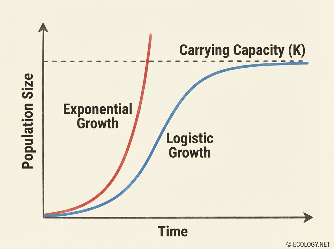
The S-curve illustrates a more realistic scenario: initial rapid growth, followed by a period where the growth rate decreases, and finally, a plateau where the population size stabilizes. This plateau represents a critical ecological concept: carrying capacity.
Carrying Capacity: Nature’s Speed Limit
The concept of carrying capacity, often denoted as ‘K’, is central to understanding logistic growth. It represents the maximum population size of a biological species that can be sustained indefinitely by a given environment, considering the available food, habitat, water, and other necessities. Once a population reaches its carrying capacity, its growth rate typically becomes zero, meaning births equal deaths, and the population size remains relatively stable.
Think of a small island with a thriving population of rabbits. Initially, with lush vegetation and few predators, the rabbits multiply rapidly. But as their numbers swell, the grass gets eaten faster than it can regrow, fresh water sources become strained, and competition for burrows intensifies. The island can only support so many rabbits before its resources are depleted. That maximum number is the island’s carrying capacity for rabbits.
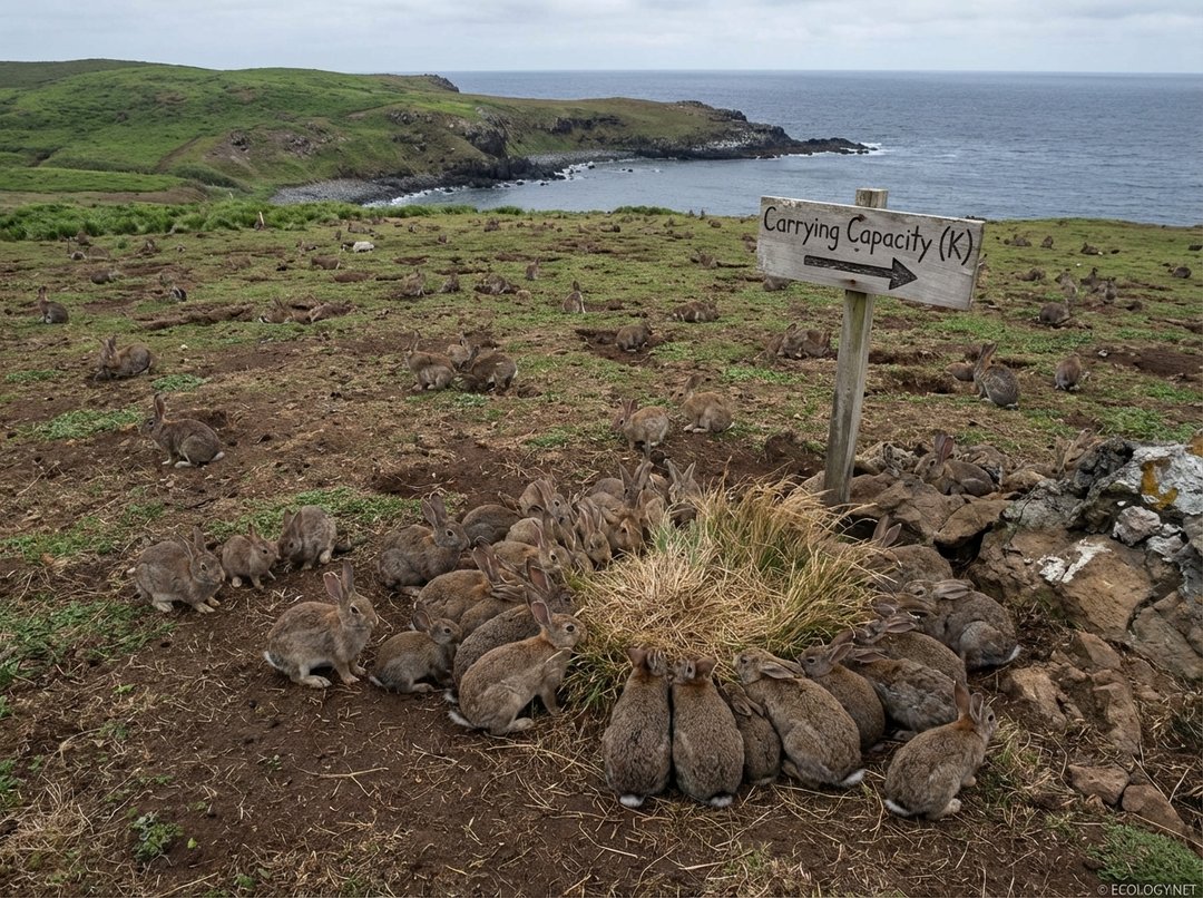
Exceeding carrying capacity can lead to a population crash, as resources become critically scarce and the environment itself may be damaged, reducing its future ability to support life.
Unpacking the S-Curve: Phases of Logistic Growth
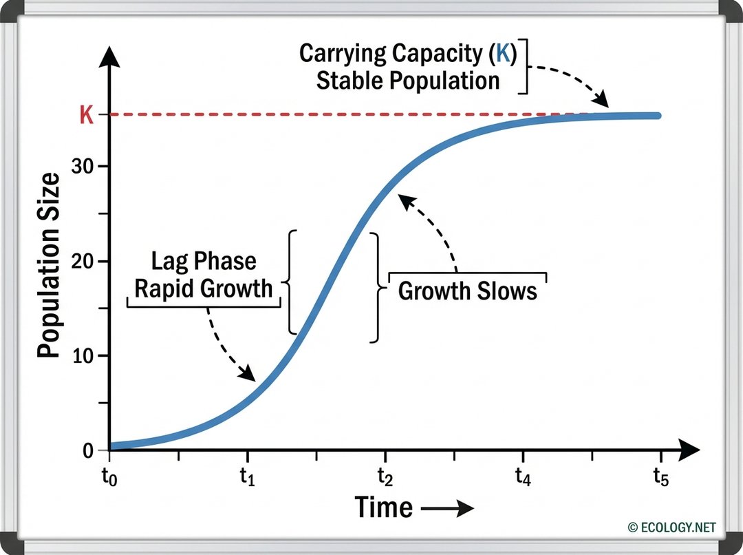
The S-shaped curve of logistic growth is not a single, uniform process, but rather a progression through distinct phases, each influenced by the population’s size relative to its environment’s carrying capacity.
Phase 1: The Lag and Rapid Ascent
At the very beginning, when a population is small and resources are abundant, the growth rate is relatively slow. This initial period is sometimes called the lag phase. Individuals might be few, and it takes time for them to find mates and reproduce. Once reproduction begins in earnest, and as long as resources remain plentiful, the population enters a period of rapid, near-exponential growth. The curve rises steeply, reflecting a high birth rate and a low death rate.
Phase 2: Growth Slows Down
As the population continues to grow, it starts to approach the carrying capacity (K) of its environment. Resources, though not yet exhausted, become less readily available. Competition for food, space, and mates increases. Waste products may accumulate. Predators might become more numerous as their food source expands. These factors begin to exert pressure, causing the population’s growth rate to decelerate. The slope of the S-curve starts to flatten, indicating that while the population is still increasing, it is doing so at a slower pace.
Phase 3: Reaching Equilibrium
Finally, the population reaches a point where its size stabilizes around the carrying capacity (K). At this stage, the birth rate and the death rate become approximately equal. The population is no longer growing significantly; instead, it fluctuates slightly above and below K, responding to minor changes in resource availability or environmental conditions. This phase represents a state of dynamic equilibrium with the environment.
What Shapes the S-Curve? Factors in Logistic Growth
The specific shape and duration of each phase in logistic growth are determined by various environmental factors, broadly categorized as density-dependent and density-independent.
Density-Dependent Factors
These are factors whose impact on population growth intensifies as the population density increases. They are the primary drivers of the slowdown in logistic growth:
- Competition for Resources: As more individuals vie for limited food, water, shelter, or sunlight, the struggle for survival intensifies, leading to reduced birth rates and increased death rates.
- Predation: Predator populations often increase in response to a larger prey population, leading to higher mortality rates for the prey.
- Disease: In denser populations, diseases can spread more easily and rapidly, causing higher mortality.
- Waste Accumulation: For some organisms, particularly microbes, the buildup of their own waste products can become toxic, inhibiting further growth.
Density-Independent Factors
These factors affect population growth regardless of the population’s density. They can impact any phase of the S-curve, often causing sudden, drastic changes:
- Natural Disasters: Events like floods, fires, earthquakes, or severe storms can decimate populations irrespective of how crowded they are.
- Climate Change: Long-term shifts in temperature or precipitation patterns can alter habitat suitability and resource availability for all individuals.
- Pollution: Environmental toxins can harm populations regardless of their density.
While density-dependent factors are crucial for the S-curve’s characteristic shape, density-independent factors can cause the carrying capacity itself to shift, or even lead to population crashes that reset the growth process.
Logistic Growth in the Wild: Real-World Tales
Understanding logistic growth is not just an academic exercise; it has profound implications for managing natural resources, conserving endangered species, and even predicting the spread of diseases.
-
Microbes in a Petri Dish
One of the classic examples of logistic growth is observed in laboratory cultures of bacteria or yeast. When a small number of cells are introduced into a fresh medium with abundant nutrients, they multiply exponentially. However, as the population grows, they consume nutrients and excrete waste products. Eventually, the nutrient supply dwindles, and waste accumulates, inhibiting further growth. The population then stabilizes at a carrying capacity determined by the initial amount of resources and the volume of the petri dish.
-
Deer on an Island
Consider a population of deer introduced to a new island with no predators and ample vegetation. Their numbers would initially soar. But as the deer population increases, they would overgraze the vegetation, leading to food shortages. This would cause a decline in birth rates and an increase in death rates, eventually stabilizing the population around the island’s carrying capacity for deer. If the carrying capacity is severely overshot, the vegetation might be permanently damaged, leading to a lower K in the future or even a population crash.
-
Human Population Dynamics (with nuance)
Applying logistic growth to human populations is complex, as our species continually innovates to overcome perceived limits. Technological advancements in agriculture, medicine, and resource extraction have historically increased Earth’s effective carrying capacity for humans. However, many ecologists argue that even with our ingenuity, there are ultimate limits to the planet’s ability to sustain an ever-growing population, particularly concerning resource depletion, pollution, and climate change. While our growth curve has not perfectly followed a simple S-shape due to these innovations, the principles of resource limitation and environmental impact remain highly relevant to our long-term sustainability.
Why Does it Matter? The Practical Power of Logistic Growth
The concept of logistic growth is more than just a theoretical model; it is a vital tool for practical applications across various fields:
- Conservation Biology: Understanding carrying capacity helps conservationists determine how many individuals of an endangered species a protected area can realistically support, guiding reintroduction programs and habitat management.
- Fisheries Management: By estimating the carrying capacity of a body of water for a particular fish species, managers can set sustainable fishing quotas, preventing overfishing and ensuring the long-term health of fish stocks.
- Pest Control: Knowledge of logistic growth can inform strategies for managing pest populations, such as introducing natural predators or limiting resources to keep their numbers below damaging levels.
- Epidemiology: The spread of infectious diseases often follows an S-shaped curve, where the initial rapid spread slows as more individuals become immune or are isolated, eventually reaching a plateau. This understanding helps public health officials predict outbreak trajectories and plan interventions.
- Resource Management: From forestry to agriculture, logistic growth models help predict sustainable harvest rates and prevent the depletion of renewable resources.
In essence, logistic growth provides a powerful framework for understanding the intricate balance between populations and their environments. It reminds us that while life strives to expand, it always operates within the boundaries set by the natural world.
From the smallest bacteria to the largest ecosystems, the S-shaped curve of logistic growth is a universal pattern, a testament to the elegant self-regulation inherent in nature. By appreciating its principles, we gain a deeper insight into the dynamics of life on Earth and equip ourselves with the knowledge to foster a more sustainable future.


